Visualizing a Single Variable in R and Python Pandas
April 24, 2015
The Data
North Carolina births
In 2004, the state of North Carolina released a large data set containing information on births recorded in this state. This data set is useful to researchers studying the relation between habits and practices of expectant mothers and the birth of their children. We will work with a random sample of observations from this data set.
Read data from URL
In R
download.file('http://www.openintro.org/stat/data/nc.RData', destfile = 'nc.RData')
load('nc.RData')
In Python
import pandas as pd
data = pd.read_csv('http://photo.etangkk.com/python/NCbirths.txt', sep='\t')
Visualizing numerical data
Histogram
Histogram is used to show the frequency across a continuous or discrete variable, its x-axis is a number line and the ordering of the bars are not interchangeable. It is useful for describing the shape of the distribution.
In R
hist(nc$fage, breaks=10, freq=TRUE, xlim=c(10, max(nc$fage, na.rm=TRUE)), ylim=c(0, 250), main='Histogram of father\'s age', xlab='Age in years')
Using ggplot2
library(ggplot2)

ggplot(data=nc, aes(x=fage)) + geom_histogram(bins=15, na.rm=TRUE) + labs(title="Histogram of father's age") + xlab('Age in years') + xlim(0, max(nc$fage, na.rm=TRUE)) + ylim(0, 200)
It can easily turn into a density plot, instead of counting the number per bin it gives the probability densities.
hist(nc$fage, breaks=15, freq=FALSE, xlim=c(10, max(nc$fage, na.rm=TRUE)), ylim=c(0, .075), main='Probability of father\'s age', xlab='Age in years')
Using ggplot2
ggplot(data=nc, aes(x=fage)) + geom_histogram(aes(y=(..density..)), col="blue", fill="yellow") + labs(title="Probability of father\'s age") + xlab('Age in years') + ylab('Probability')
In Python
import matplotlib.pyplot as plt
%matplotlib inline
ax = data['fage'].plot(kind='hist', bins=10, xlim=[10, data['fage'].max()], ylim=[0, 200])
ax.set_title('Histogram of father\'s age')
ax.set_xlabel('Age in years')
ax.set_ylabel('Frequency')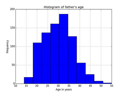
Using seaborn
import seaborn as sns
f, ax = plt.subplots(figsize=(6, 4));
sns.distplot(data['fage'].dropna(), hist=True, kde=False, rug=False, bins=10);
ax.set(xlim=(0, data['fage'].max()), ylabel="Frequency", xlabel="Age in years", title="Histogram of father\'s age")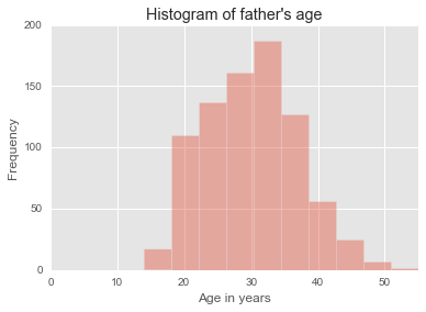
ax = data['fage'].plot(kind='hist', bins=15, normed=True, xlim=[10, data['fage'].max()])
ax.set_title('Probability of father\'s age')
ax.set_xlabel('Age in years')
ax.set_ylabel('Density')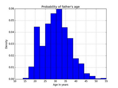
Using seaborn
import seaborn as sns
f, ax = plt.subplots(figsize=(6, 4));
sns.distplot(data['fage'].dropna(), hist=True, kde=True, rug=False, bins=10);
ax.set(xlim=(0, data['fage'].max()), ylabel="Density", xlabel="Age in years", title="Probability of father\'s age")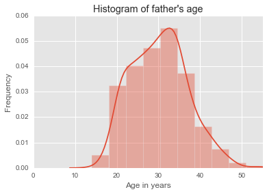
Histogram and bin width
The choice of bin width can alter the story the histogram is telling.

Density plot
Density plots are usually a more effective way to view the distribution of a continuous variable.
plot(density(nc$fage, na.rm=TRUE), add=TRUE, main="Density of father\'s age", xlab='Father age')
Using ggplot2
ggplot(data=nc, aes(x=fage)) + geom_density(alpha=.2, fill="red") + labs(title="Probability of father\'s age") + xlab('Age in years') + ylab('Probability')
In Python Using seaborn
import seaborn as sns
f, ax = plt.subplots(figsize=(6, 4));
sns.distplot(data['fage'].dropna(), hist=False, kde=True, rug=False, bins=10);
ax.set(xlim=(0, data['fage'].max()), ylabel="Density", xlabel="Age in years", title="Density of father\'s age")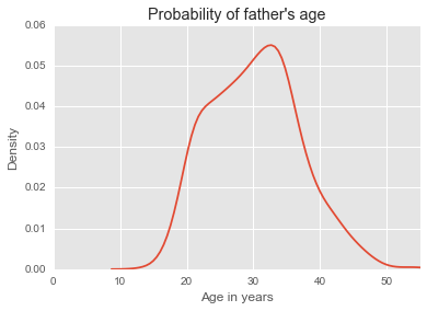
Box plot
Boxplot is useful for highlighting outliers, median, and interquartile range (IQR).
In R
boxplot(nc$gained, horizontal=TRUE, xlab='Weight gained by mother during pregnancy in pounds')
Using ggplot2
ggplot(nc, aes(x=factor(0), y=gained)) + geom_boxplot() + xlab("") + ylab("Weight gained by mother during pregnancy in pounds") + scale_x_discrete(breaks=NULL) + coord_flip()
In Python
ax = data['gained'].plot(kind='box', vert=False)
ax.set_xlabel('Weight gained by mother during pregnancy in pounds')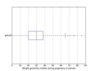
Using seaborn
import seaborn as sns
f, ax = plt.subplots(figsize=(6, 4));
sns.distplot(data['fage'].dropna(), hist=False, kde=True, rug=False, bins=10);
ax.set(xlim=(0, data['fage'].max()), ylabel="Density", xlabel="Age in years", title="Density of father\'s age")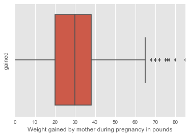
Visualizing categorical data
Frequency table
Frequency table is the easiest way to see what occurs most often in a set of data.
In R
mytable <- table(nc$whitemom, exclude=NULL)
print(mytable)
##
## not white white <NA>
## 284 714 2Table of proportions displays the relative frequency.
prop.table(mytable)##
## not white white <NA>
## 0.284 0.714 0.002In Python
data['whitemom'].value_counts()## white 714
## not white 284
## dtype: int64There is no table of proportions in Python, I’ve written the following function to generate a frequency table with percentage in Python.
def freq_table(df, var, rmna=False):
    if rmna is True:
        df[var] = df[var].replace(np.nan, 'NaN')
    table = pd.DataFrame(df.groupby(var)[var].count())
    table['Freq'] = list(map(lambda x: round(x, 2), table[var] / float(table.sum()) * 100))
    table.columns = ['Counts', 'Frequencies']
    print table
    return table

t = freq_table(data, 'whitemom')
freq_table(data, 'whitemom', True)
## Counts Frequencies
## whitemom
## not white 284 28.46
## white 714 71.54
## Counts Frequencies
## whitemom
## NaN 2 0.2
## not white 284 28.4
## white 714 71.4Bar plot
Barplot is analogous to histogram but for categorical variables.
In R
par(mfrow=c(1, 2))
counts <- table(nc$lowbirthweight)
percent <- prop.table(counts)
barplot(counts, width=3, horiz=TRUE, main='Low birth weight distribution')
barplot(percent, width=6, main='Probability of low birth weight')
Using ggplot2
p1 <- ggplot(data=nc, aes(x=lowbirthweight)) + geom_bar(col="blue", fill="yellow", alpha=.2) + labs(title="Low birth weight distribution")

library(scales)
p2 <- ggplot(data=nc, aes(x=lowbirthweight)) + geom_bar(aes(y=round((..count..)/sum(..count..)*100, 2)), fill='yellow') + geom_text(aes(y = ((..count..)/sum(..count..)*100), label=scales::percent((..count..)/sum(..count..))), stat="count", vjust = -0.25) + labs(title="Probability of low birth weight", y="Percent", x="Birth Weight") + coord_flip()

library(gridExtra)
grid.arrange(p1, p2, ncol=2, nrow=1)
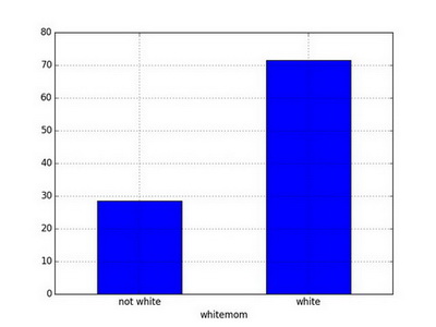
In Python
ax = t['Counts'].plot(kind='barh')

ax = t['Frequencies'].plot(kind='bar')
ax.set_xticklabels(t.index, rotation=0)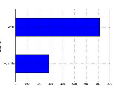
Using seaborn
import seaborn as sns
sns.countplot(data['whitemom']);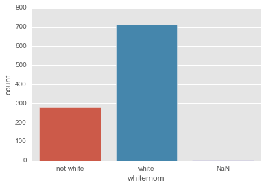
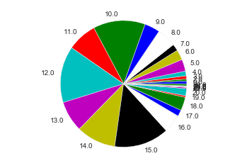
Pie chart
Barplot is analogous to histogram but for categorical variables.
In R
library(plotrix)
library(dplyr)

nc$visits_bucket <- cut(nc$visits, breaks=seq(0,30,10), include.lowest=TRUE)
nc$visits_bucket <- ifelse(is.na(nc$visits_bucket), "NA", nc$visits_bucket)

d1 <- group_by(nc, visits_bucket) %>% summarise(cnt=length(visits_bucket), pct=length(visits_bucket)/length(nc$visits_bucket)*100)

par(mfrow=c(1, 2))
#counts <- table(nc$visits_bucket)
#percent <- prop.table(counts)
pie(d1$cnt, labels=d1$visits_bucket, main="Pie chart of visits")
pie3D(d1$cnt, labels=d1$visits_bucket, explode=0.1, main="3D Pie chart of visits")
Using ggplot2
g1 <- ggplot(d1, aes(x="", y=cnt, fill=visits_bucket)) + geom_bar(stat="identity") + coord_polar(theta="y", start=0) + guides(fill=guide_legend(title="Visits", ncol=4))
g1 <- g1 + geom_text(aes(y = d1$cnt/3 + c(0, cumsum(d1$cnt)[-length(d1$cnt)]), label=d1$pct)) + ggtitle("Pie chart of visits")
g1 <- g1 + theme(legend.position="top", axis.text=element_blank(), axis.title = element_blank(), axis.ticks = element_blank())

print(g1)
In Python
sums = data.groupby('visits').size()
axis('equal');
pie(sums, labels=sums.index);